Technical-Charts
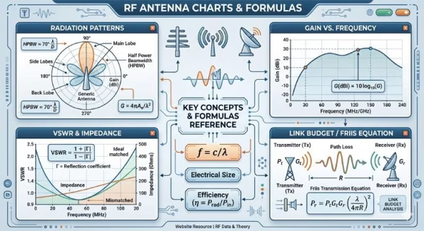
RF Antenna Technical Charts & Performance Metrics
Technical charts serve as the primary diagnostic and evaluative tools for RF engineers analyzing antenna performance across varying operational profiles. Principal among these is the polar radiation pattern plot, which maps 360-degree spatial signal distribution to visually define the main lobe, sidelobes, back lobe, and half-power beamwidth (HPBW). Complementing this spatial data, Return Loss (S11) and Voltage Standing Wave Ratio (VSWR) frequency sweeps quantify impedance matching efficiency, explicitly illustrating how well the antenna transfers energy across its designated bandwidth. Gain-versus-frequency line graphs track absolute radiation intensity (dBi) over the operational band, providing critical data for system link budget calculations. For complex phased arrays and multi-band deployments, co-polarization and cross-polarization isolation plots reveal the antenna's vulnerability to signal interference and polarization mismatch. Ultimately, these interrelated graphical matrices convert abstract electromagnetic behavior into precise, actionable datasets, enabling procurement officers and system integrators to confidently verify mission-critical specifications.
RF Power Conversion Table: dBm to Watts
For the RF Engineers, a conversion table is a fundamental tool for engineers to quickly translate between logarithmic power levels (dBm) and linear power levels (Watts).
| Power (dBm) | Power (Watts) | Engineering Context |
| 60 dBm | 1000 W (1 kW) | High-power broadcast transmitters. |
| 53 dBm | 200 W | High-gain base station amplifiers. |
| 50 dBm | 100 W | Standard high-power RF systems. |
| 47 dBm | 50 W | Large cellular macrocells. |
| 43 dBm | 20 W | Typical outdoor cellular sectors. |
| 40 dBm | 10 W | High-performance RF amplifiers. |
| 37 dBm | 5 W | Medium-range wireless links. |
| 33 dBm | 2 W | Common for specialized military antennas. |
| 30 dBm | 1 W | Standard limit for many Wi-Fi routers. |
| 27 dBm | 500 mW | Industrial IoT and telemetry. |
| 23 dBm | 200 mW | Standard mobile device output. |
| 20 dBm | 100 mW | Low-power industrial transmitters. |
| 17 dBm | 50 mW | Typical Bluetooth Class 1. |
| 10 dBm | 10 mW | Short-range telemetry / IoT. |
| 7 dBm | 5 mW | Low-power sensors. |
| 3 dBm | 2 mW | Doubling of the 0 dBm reference. |
| 0 dBm | 1 mW | The Fundamental Reference Point. |
Mental Math Cheat Sheet: When a table is not available, engineers use the Rule of 3s and 10s to estimate values:
- +10 dB: Increases power by 10 times
- -10 dB: Decreases power to 1/10th
- +3 dB: Approximately doubles the power
- -3 dB: Approximately halves the power
- Example: To find 13 dBm, start at 10 dBm (10 mW) and add 3 dB. Doubling 10 mW gives you 20 mW.
Return Loss vs. VSWR Conversion Table
In the study of RF systems, Return Loss and Voltage Standing Wave Ratio (VSWR) are two different ways to measure the efficiency of power delivery from a transmitter to an antenna. Both metrics describe the "match" between the transmission line and the load, indicating how much energy is reflected back toward the source.
This table provides a quick reference for understanding how much power is lost due to impedance mismatch. For the RF Engineers, a conversion table is a fundamental tool for engineers to quickly translate between logarithmic power levels (dBm) and linear power levels (Watts).
| VSWR | Return Loss (dB) | Reflection Coefficient (Γ) | Power Reflected (%) | Mismatch Loss (dB) |
| 1.01:1 | 46.06 | 0.005 | 0.002% | 0.0001 |
| 1.05:1 | 32.26 | 0.024 | 0.06% | 0.003 |
| 1.10:1 | 26.44 | 0.048 | 0.23% | 0.010 |
| 1.20:1 | 20.83 | 0.091 | 0.83% | 0.036 |
| 1.30:1 | 17.69 | 0.130 | 1.70% | 0.075 |
| 1.50:1 | 13.98 | 0.200 | 4.00% | 0.177 |
| 2.00:1 | 9.54 | 0.333 | 11.1% | 0.512 |
| 3.00:1 | 6.02 | 0.500 | 25.0% | 1.249 |
| 5.00:1 | 3.52 | 0.667 | 44.4% | 2.553 |
| 10.0:1 | 1.74 | 0.818 | 66.9% | 4.807 |
Understanding the Metrics
VSWR (Voltage Standing Wave Ratio): VSWR is a linear ratio that describes the standing wave resultant from the interference of the incident wave and the reflected wave. An ideal VSWR is 1.0:1, meaning no power is reflected. Most professional antenna systems aim for a VSWR below 1.5:1 or 2.0:1.
Return Loss (dB): Return Loss is the ratio of incident power to reflected power, expressed in decibels. A higher positive value (e.g., 20 dB) indicates a better match, as more power is "lost" to the antenna rather than returning to the source. A lower value (e.g., 3 dB) indicates a poor match, meaning nearly half the power is being reflected back.
Mechanical Down-tilt Reference Table
In cellular and RF network planning, adjusting the Antenna Down-tilt relative to the Mounting Height is a critical process for controlling the cell radius, reducing interference with neighboring cells, and maximizing signal strength within the intended coverage area.
This relationship is governed by the distance from the tower to the target coverage point and the height difference between the antenna and the receiver.
The following table provides the required tilt angles (in degrees) to target a specific distance based on various mounting heights. These values are calculated using basic trigonometry: Angle = arctan(Height/Distance).
| Height (m) | 500m Distance | 1km Distance | 2km Distance | 5km Distance |
| 10m | 1.15° | 0.57° | 0.29° | 0.11° |
| 20m | 2.29° | 1.15° | 0.57° | 0.23° |
| 30m | 3.43° | 1.72° | 0.86° | 0.34° |
| 45m | 5.14° | 2.58° | 1.29° | 0.52° |
| 60m | 6.84° | 3.43° | 1.72° | 0.69° |
Key Concepts in Down-tilting
- Mechanical Tilt: Physically angling the antenna bracket. This shifts the entire radiation pattern, including the back-lobe, which can sometimes lead to coverage gaps directly behind the tower.
- Electrical Tilt: Adjusting the phase of the individual elements within the antenna array. This tilts the main beam uniformly in all horizontal directions without changing the physical position of the antenna housing.
- The Null Fill: When high tilt angles are used (especially on tall towers), "nulls" in the radiation pattern can cause "dead zones" close to the base of the tower. High-quality antennas include null-fill technology to prevent this.
- Impact of Height on Coverage
| Height Change | Effect on Coverage | Effect on Interference |
| Increasing Height | Larger footprint, better line-of-sight (LOS). | Higher risk of overshooting and interfering with distant cells. |
| Increasing Tilt | Reduced cell radius, stronger signal in-building. | Clears frequency reuse for neighboring sectors. |
RF Connector Types Vs Frequency Range Table
Selecting the correct RF connector is critical to maintaining signal integrity and preventing leakage, especially as systems move into higher frequency bands like Ku, Ka, and Q/V bands. Each connector type has a "cutoff frequency" where the signal begins to degrade or modes other than the primary TEM mode begin to propagate.
| Connector Type | Typical Frequency Range | Max Cutoff Frequency | Best Use Case |
| UHF (PL-259) | DC – 300 MHz | ~500 MHz | HF/VHF Amateur Radio, CB. |
| BNC | DC – 4 GHz | 12 GHz (Specialized) | Test equipment, Video, Low-power RF. |
| TNC | DC – 11 GHz | 18 GHz | Tactical radio, Avionics (Vibration resistant). |
| N-Type | DC – 11 GHz | 18 GHz | Base stations, Outdoor antennas, High power. |
| SMA | DC – 18 GHz | 26.5 GHz | PCB prototyping, Wi-Fi, SATCOM. |
| 2.92mm (K) | DC – 40 GHz | 40 GHz | Millimeter Wave (mmWave), High-speed digital. |
| 2.40mm | DC – 50 GHz | 50 GHz | Advanced radar, 5G research. |
| 1.85mm (V) | DC – 67 GHz | 67 GHz | Q/V Band Satellite, Automotive Radar. |
| 1.00mm | DC – 110 GHz | 110 GHz | Terahertz imaging, experimental physics. |
Key Selection Factors
- Impedance Matching: Most RF connectors are designed for 50 Ohms impedance. Using a 75 Ohms connector (common in video/cable TV) in a 50 Ohms system will cause significant VSWR issues.
- Power Handling: Larger connectors like N-Type or 7/16 DIN can handle hundreds of Watts. Small connectors like SMA are typically limited to low-power applications (under 50-100W depending on frequency).
- Durability: Threaded connectors (N-Type, SMA, TNC) provide better shielding and stability under vibration than "push-on" or bayonet styles (BNC).
RF Connector Power Handling (Watts) @ Frequency Band Table
The power handling capability (measured in Watts) of an RF connector is not a single fixed value; it decreases as the frequency increases. This is due to dielectric heating and "skin effect" losses that generate heat within the connector.
The following table provides the Average Power Handling (CW - Continuous Wave) for standard 50 Ohms connectors at sea level and room temperature (25 Degrees Celsius).
| Connector Type | @ 100 MHz | @ 1 GHz | @ 10 GHz | Peak Voltage (V) |
| 7/16 DIN | 5,000 W | 1,500 W | N/A | 2,700 V |
| N-Type | 1,000 W | 300 W | 80 W | 1,500 V |
| TNC | 500 W | 150 W | 40 W | 500 V |
| BNC | 400 W | 100 W | N/A | 500 V |
| SMA | 150 W | 50 W | 15 W | 335 V |
| 2.92mm (K) | 100 W | 30 W | 10 W | 250 V |
| SSMA | 60 W | 20 W | 5 W | 170 V |
| MCX / MMCX | 50 W | 15 W | N/A | 170 V |
Critical Derating Factors
When designing a system for the Technical Library, users should be aware that the "Catalogue Rating" of a connector must be derated based on environmental conditions:
- VSWR (Reflected Power): High VSWR creates "voltage standing waves" that increase the peak voltage and localized heating at the connector interface. A VSWR of 2.0:1 can reduce power handling by roughly 10-15%.
- Altitude (Air Density): As altitude increases, the breakdown voltage of air decreases. For aerospace or high-altitude ground stations, power ratings must be significantly reduced to prevent arcing or corona discharge.
- Temperature: If the ambient temperature is 70 Degrees Celsius instead of 25 Degrees Celsius the connector's ability to dissipate heat is reduced. A common rule of thumb is to derate power by 40-50% for high-temperature environments.
- Modulation (Peak vs. Average): Pulse-based signals (like Radar) have very high Peak Power but low Average Power. Ensure the connector's Voltage Rating can handle the peaks, even if the average power is within limits.
- For Base Stations (High Power): Always use 7/16 DIN or 4.3-10 connectors. These are designed to minimize PIM (Passive Intermodulation) and handle the high heat of continuous transmission.
- For General Outdoor Use: The N-Type connector remains the industry standard for its balance of ruggedness, weatherproofing, and respectable power handling up to 11 GHz.
- For Miniature Tech: Use SMA only for low-power drive signals or receive-only paths where power levels are typically below 10-20 Watts.
Standard Rectangular Waveguide Frequency Chart
Waveguides are physical structures—typically hollow metallic pipes—used to guide electromagnetic waves at high frequencies where coaxial cables become too lossy. They act as high-pass filters, meaning they only support wave propagation above a certain "cutoff frequency".
The table below lists the standard Rectangular Waveguide designations (EIA WR-series) and their optimal operating frequency ranges for the dominant TE10 mode.
| EIA Designation | Frequency Range (GHz) | Cutoff Frequency (GHz) | Common Band Name |
| WR-2300 | 0.32 – 0.49 | 0.257 | UHF Band |
| WR-975 | 0.75 – 1.12 | 0.605 | L Band |
| WR-650 | 1.12 – 1.70 | 0.908 | L Band |
| WR-430 | 1.70 – 2.60 | 1.372 | S Band |
| WR-284 | 2.60 – 3.95 | 2.078 | S Band |
| WR-187 | 3.95 – 5.85 | 3.152 | C Band |
| WR-137 | 5.85 – 8.20 | 4.301 | C Band |
| WR-90 | 8.20 – 12.4 | 6.557 | X Band |
| WR-62 | 12.4 – 18.0 | 9.488 | Ku Band |
| WR-42 | 18.0 – 26.5 | 14.047 | K Band |
| WR-28 | 26.5 – 40.0 | 21.071 | Ka Band |
| WR-19 | 40.0 – 60.0 | 31.357 | U Band |
| WR-10 | 75.0 – 110.0 | 59.015 | W Band |
Key Technical Concepts
- Cutoff Frequency (fc): The lowest frequency at which a specific mode can propagate. For a rectangular waveguide of width a, the dominant mode cutoff is fc = c / 2a
- Operating Range: To avoid signal distortion and multiple mode interference, waveguides are typically used within 125% to 190% of their cutoff frequency.
- Power Handling: Waveguides can handle significantly higher power than coaxial cables because they are air-filled and lack a center conductor, which reduces dielectric heating and prevents arcing.
- Attenuation: Above the cutoff frequency, waveguides offer extremely low attenuation, making them the standard for high-power radar and satellite ground station uplinks.
Waveguide vs. Coaxial Selection
| Feature | Coaxial Cable | Waveguide |
| Bandwidth | Very Wide (DC to GHz) | Narrow (Limited by modes) |
| Power Capacity | Low to Medium | Very High |
| Loss (Attenuation) | High at high frequencies | Very Low |
| Physical Flexibility | Flexible | Rigid (Requires precision bends) |
| Cost | Lower | Higher (Precision machining) |
